Fractals

Have you ever noticed how a tree has trunks with branches connected to ends, and each one of those branches has branches at its end, and those branches have more branches and so on? And now each of this branch of the whole tree, its sub-branch, its sub-sub-branch look similar to the whole tree itself.

Now, take a look at this carpet. It obviously isn’t just a carpet. This special carpet has little carpets inside of it. And those carpets have even smaller carpets.

The Sierpinski carpet zoomed up to the sixth iteration.

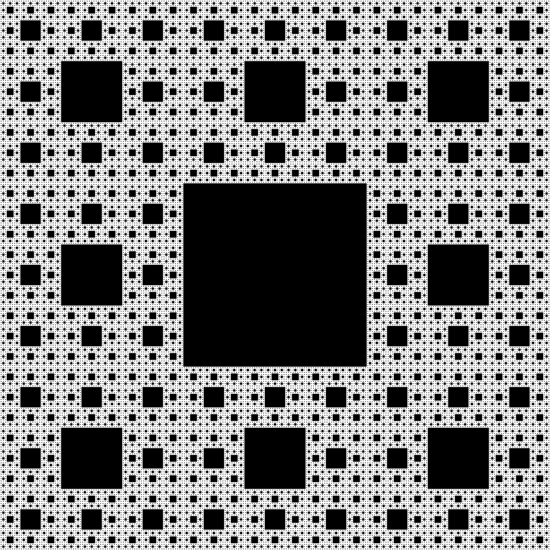
What you see here and in the example of the tree above is a fractal, a pattern that keeps repeating itself infinitely either exactly or almost exactly at smaller and smaller scales.

It is somewhat mesmerizing to infinitely zoom in into a fractal (XaoS.js). You expect it to finally take a final simple shape but it just keeps going on and on.

---

Fractals can be found everywhere in nature. Take snowflakes, for example, ice crystals that branch out into repeating structures that extend infinitely. Or take hurricanes, self-organizing spirals. Far from being exceptions, highly irregular objects like fractals are surprisingly commonplace in nature.

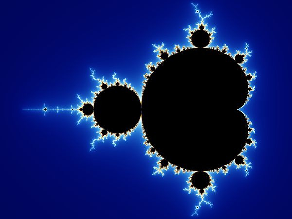
The Mandelbrot Set

The father of fractal geometry, Benoit B. Mandelbrot, had a breakthrough when he discovered the Mandelbrot set is given by the complex function:

\(f_c = z^2 + c\)

at all complex points c where the function remains bounded.

The Mandelbrot set. Points where the function doesn’t “explode” are shaded black.

Now, fractals aren’t just an idea of self-similarity—they go deeper than that. They are, maybe a bit more accurately, a mathematician’s desire to capture roughness in geometry. A straight line might be self-similar but it is not a fractal. What makes fractals special is how they break away from the neat rules of Euclidean geometry.

An attempt at describing this roughness is found in the fractal dimension. But first I would like to talk more about what exactly a dimension is.

Dimension

Dimension can be defined in a variety of different ways in a variety of different fields.

Dimension of a mathematical space, at it’s most simplest sense, is defined as the minimum number of numbers required to determine the position of a point in said mathematical space. This is the most basic definition of a dimension, which is specific to mathematics. To define the dimension of a fractal, however, this idea does not suffice.

Fractal Dimension

To proceed, we notice one crucial difference between standard euclidean figures and fractals, in how they 'scale'. Simple Euclidean figures scale like so:

A line, when its scaled down, it shrinks to half of its length, the square half of its area and the cube half of its volume. This can be called as the scaling factor.

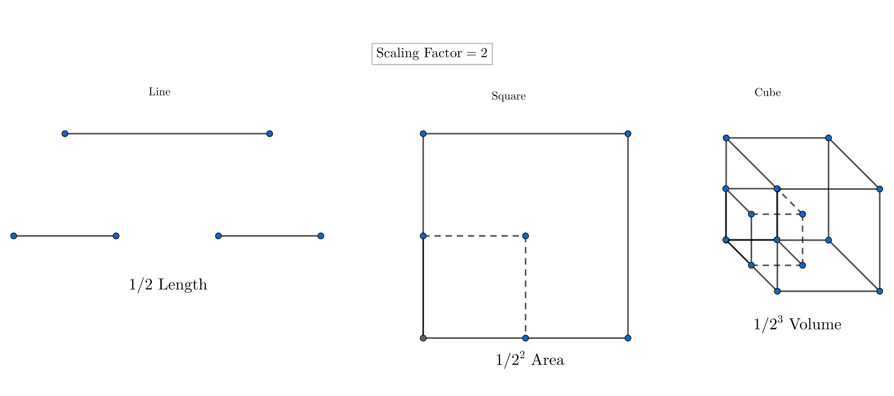
If a fractal's one-dimensional lengths are all doubled, the spatial content of the fractal scales by a power that is not necessarily an integer. This is the fractal dimension.

A fractal, such as the Sierpinski triangle, can shrink down into 3 thirds with a scale factor of 12. That is, each constituent is half of the parent triangle. Or 2ᴰ constituent triangles make one whole, where D is the fractal dimension. Since, there are 3 constituents, 2ᴰ will equal 3, giving D = 1.585. D is the fractal dimension, given by, again, Mandelbrot who was motivated by the Hausdorff dimension.

Creating Fractals

But how do we actually create fractals?

We can start with drawing. Suppose we want to draw the Koch snowflake:

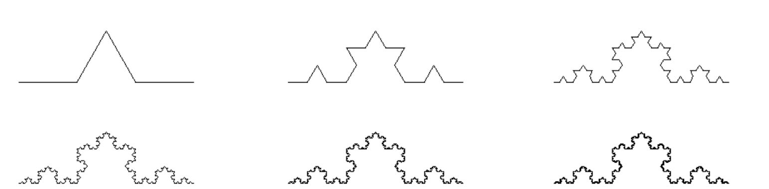
As you might have noticed, a fractal is just an iteration. We start with a single small “bump”. Then we take all the 4 lines and bump them. Then we repeat, take each line and make a small bump.

That is: by starting with a triangular bump and then iterating the four same scaling transformations n times, we get the nᵗʰ level of the Koch curve.

So if we know the first few levels of a fractal, we can find the (affine) transformations that produce level 2 from level 1 and verify that these same transformations generate level 3 from level 2, allowing us to identify the underlying iterative process used to generate that fractal.

Now, suppose we have a set of transformations that, for any level n, convert the structure at level n of a fractal to the next level. Because fractals are self-similar each level is similar to the whole. Hence, as n→∞, these transformations will necessarily map out the fractal itself. This idea can be used to generate fractals using certain systems called iterated function systems.

---

From the previous section we saw that fractals are just iterations upon iterations of certain transformations. Let us take one such transformation, f, as a function that spits out the midpoint of two input points.

\(f(P_1,P_2) = \frac{P_1+ P_2}{2}\)

Doing this for n = 3 individual points iteratively can be condensed to:

\(H(P)=\bigcup_{i=1}^{3}f_i(P)\)

where H is called the Hutchinson operator. A few thousand iterations eventually give us the Sierpinski triangle (Algorithms Archive):

There is a more algebraically rigorous way to define an IFS as a group of affine transformation applied repeatedly to a fractal as a group of points. A typical affine transformation to generate the Sierpinski triangle looks like this:

\({f_1}({\bf{x}}) = \left[ {\begin{matrix} {1/2} & 0 \\ 0 & {1/2} \\ \end{matrix}} \right]{\bf{x}}\)

\({f_2}({\bf{x}}) = \left[ {\begin{matrix} {1/2} & 0 \\ 0 & {1/2} \\ \end{matrix}} \right]{\bf{x}} + \left[ {\begin{matrix} {1/2} \\ 0 \\ \end{matrix}} \right]\)

\({f_3}({\bf{x}}) = \left[ {\begin{matrix} {1/2} & 0 \\ 0 & {1/2} \\ \end{matrix}} \right]{\bf{x}} + \left[ {\begin{matrix} {1/4} \\ \sqrt3/4 \\ \end{matrix}} \right]\)

Here are more fractals built using an IFS: https://larryriddle.agnesscott.org/ifskit/gallery/gallery.htm.

For further reading and watching, I suggest:

1. https://larryriddle.agnesscott.org/ifs/ifs.htm

2. A very nice video on affine transformations: Leios Labs: What are affine transformations?

3. https://mathworld.wolfram.com/LindenmayerSystem.html

4. https://www.algorithm-archive.org/contents/affine_transformations/affine_transformations.html

Chaos Game

We can construct fractals the other way too. We can pick a point randomly and have a computer randomly decide which point to pick as the second from A,B, and C. Then, iteratively, the next point is given by p_n, where v is one of A,B, or C.

\(p_n = \frac{p_{n-1} + v}{2}\)

What we eventually get is, again, the Sierpinski triangle.

There are tons of links on the internet for playing around with this “chaos game”. My personal favorite is the one on shodor.org.

What is interesting is that, after a couple initial iterations, the empty spaces in the figure obtained never get filled. As iterations increase, the group of points continually converge or get attracted to the Sierpinski Triangle. The Sierpinski Triangle is, hence, called the attractor. This chaos game plots points in such a manner that it limits children of the next point to be within the confines of the attractor.

So once, as result of the chaos game, a children point touches what is going to be the attractor, future children stay within the (future) confines of the attractor.

Of course, we are not limited to three points, neither are we limited to finding the midpoint between pₙ₋₁ and v. We can change r and increase the size of v to include more vertices.

The obvious question is, of course, why? Why does any chaos game converge to an attractor?

While a full proof would be too lengthy for this article (see: Why does the chaos game converge to the Sierpinski triangle?), we can intuitively understand that each step in the chaos game corresponds to a linear transformation that moves a point closer to one of the triangle's vertices. These transformations are contractions, meaning they reduce the distance between points at each iteration, eventually converging to the attractor. In other words, it is the unique set that remains invariant (doesn’t change) under repeated application of these transformations.

Chaos Theory

The chaos game shows how random choices can create beautiful, organized shapes (like fractals). This is a small example of a bigger idea in math, concerned with the field of chaos theory: even in messy, unpredictable systems, there’s often hidden order.

To begin, I'd like to briefly digress. I would like to talk about universality. Take, for example, the two body problem. It’s solvable, and that to quite satisfactorily, it’s easy to understand, it’s predictable. Then comes the three body problem, it is often not at all predictable, and doesn’t have a universal solution.

But now keep increasing this n, the number of objects. First it gets worse, horribly worse, becoming infinitely unpredictable, even though it already was that much unpredictable. But there comes a point where you see simple clusters of objects, galaxies, composed of hundred thousand millions of stars, forming into similar and familiar patterns.

A motion of a galaxy, the galactic rotation curve, is very much predictable, and this macroscopic structure is not at all related to the microscopic stars composing the galaxy.

This emergence of order, despite the underlying chaos, illustrates universality—where complex, unpredictable systems give rise to familiar, predictable patterns at larger scales.

Chaos theory, as its called, is the science of surprises. It deals with nonlinear dynamical systems. In a nonlinear system, changes in input do not result in proportionate changes in output. Dynamical indicates that the state of the system continuously changes in response to internal or external factors.

Chaotic systems are highly sensitive to initial conditions. Edward Lorenz, the father of chaos theory, described chaos as “when the present determines the future but the approximate present does not approximately determine the future.”

Many chaotic systems as we will see in the following section have fractal representations.

Logistic map

Consider:

\(x_{n+1}=rx_n(1-x_n).\)

This is a difference equation called the logistic map.

The logistic map is a discrete version of the logistic equation:

\(\frac{d}{dx}f(x)=rf(x)(1-f(x))\)

The logistic equation was originally used to model population systems in biology, and so, we can think of f(x) as a continuous function, modelling population. The logistic map, whereas, maps the population value at equal time steps from n = 0 to 1 to 2 and so on.

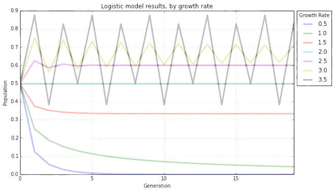
The obvious thing that we can do seeing the difference equation is vary r.

Notice how for lower r the lines converge to a stable value but as r goes higher the system tends toward a certain periodicity. For example, r=3, converges slowly to a certain value but the line at r=3.5 just bounces around.

Let us call these fixed point(s), (an) attractor(s). An attractor is the value, or set of values, that the system approaches over time. A chaotic system has a strange attractor, around which the system oscillates over time.

This attractor is just like the one we saw in the chaos game.

The attractor can be modeled against the growth rate to give out a bifurcation diagram. Notice how, beyond ~3.6, the bifurcations continually increase, leading to chaos. This is known as periodic-doubling route to chaos, where each bifurcation splits into two.

The bifurcation diagram. Each vertical line at a certain r, when it intersects, with the diagram leads to the attractor for that r.

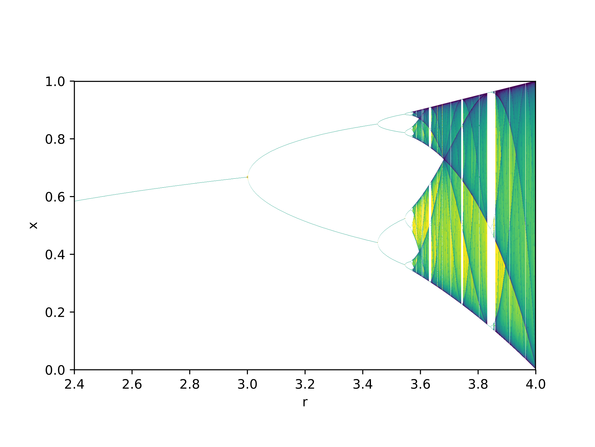
This bifurcation diagram is, as you might have noticed, a fractal. But something that you might have not noticed is this:

An isometric view of the logistic map and the Mandelbrot set.

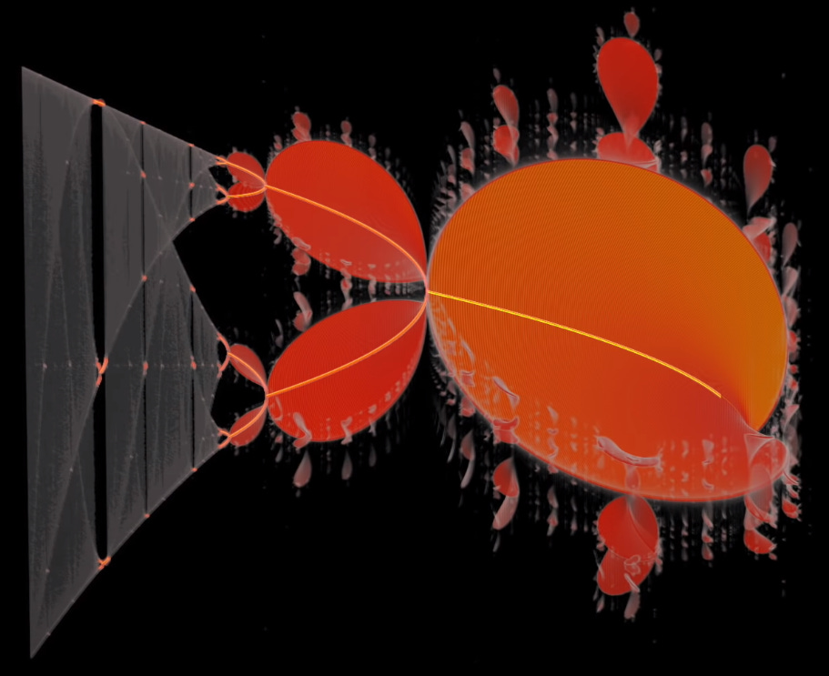
The logistic map is kind of a third dimension, a part of the Mandelbrot set. Mathematically, we can justify this: both the logistic map and the Mandelbrot set are quadratic maps and a change of variable can allow the logistic map to be re-coded into the form of the Mandelbrot set.

Now, back to the bifurcation diagram, we take the limit of the ratio of distances between consecutive lengths between bifurcations:

\(\lim_{i\rightarrow\infty}\frac{L_i}{L_{i+1}}=\delta\approx4.669\)

This δ is the Feigenbaum constant. This same constant appears, seemingly out of nowhere, in the limiting ratio of the diameters of successive circles on the real axis in the Mandelbrot set.

So, we see that the same constant appears in two different representations which earlier seemed unrelated at first. This is just universality, which restated, is the observation that seemingly different systems can exhibit the same qualitative behavior.

---

Chaotic-fractal systems show up in a bunch of real-world stuff from faucets to heart rates and to random number generators, showing how complex random processes follow sensitive but still deterministic patterns.

A lot more can be said about the logistic map and chaos theory as a whole. If you want to dive deeper and learn more:

1. An introduction: Veritasium, This equation will change how you see the world (the logistic map)

2. The book on dynamical systems: Nonlinear Dynamics and Chaos: With Applications to Physics, Biology, Chemistry, and Engineering by Steven Strogatz

3. The logistic map and Mandelbrot set in more detail: Desdenova, Is the logistic map hiding in the Mandelbrot set?

4. Numberphile’s recent video on a 1.58-dimensional object

5. Somewhat unrelated but still interesting: 2swap, Mandelbrot's evil twin

Further suggested reading:

1. “The Fractal Geometry of Nature. By Benoit B. Mandelbrot.” The American Mathematical Monthly 91

2. “Chaos: Making a New Science”. By James Gleick